We seek to find the image \(f\) which minimizes the following given an input image \(g\)

\[O(f) = \underset{f}{\max}\|\vec g-(M\vec f)\|_2^2 +\lambda \|\Gamma\vec f\|_2^2\]

Here \(M\) is a low-pass filtering operator, \(\Gamma\) is a high-pass filter and \(\lambda\) is a regularization parameter, yet to be determined. We see that the gradient of the objective function is given as

\[\frac{\partial O}{\partial \vec f} = -M^T(\vec g-M\vec f) +2\lambda \Gamma^T\Gamma \vec f\]

We observe that any optimal \(f\) must be stationary; that is it must have gradient zero. From this we obtain the following necessary condition to optimality.

\[\frac{\partial O}{\partial \vec f} = 0 \Leftrightarrow \left(M^TM+ 2\lambda \Gamma^T\Gamma\right) \vec f = M^T \vec g\]

Now for the sake of putting together concepts personally I have chosen to solve this directly. The theory is very pretty but the practicality of it requires some nitpicking with padding. We note that \(K=kk^T\) is given as a separable kernel in each of the problems. Now the circulant convolution of \(f\) and a \(1\)-dimensional kernel is given as follows

\[f\ast_c k = \textit{circulant}(k^T) f\]

Where \(\textit{circulant}(k^T)\) is a special Toeplitz matrix, known as a ‘circulant’ matrix. Then the non-circular convolution is given by padding \(k\) sufficiently. Let \(f\in \mathbb{R}^{n\times p}\) and \(\textit{length}(k)=m\), we define the following functions \(\textit{circulantPad}(k^T) = \textit{circulant}([k,0_{1 \times (\max(n,p)+\lfloor m/2 \rfloor + 1)}])\) and pad \(f\) first by \(\textit{padSquare}(f)\) which appends rows or columns of trailing \(0\)s such that \(f\) is square, then

\[\textit{pad}(f) = \begin{bmatrix}0_{\lfloor m/2\rfloor\times\lfloor m/2\rfloor} & 0_{\lfloor m/2\rfloor\times \max(n,p) } & 0_{ \lfloor m/2\rfloor\times m+1 }\\ 0_{\max(n,p)\times\lfloor m/2\rfloor} & \textit{padSquare}(f) & 0_{\max(n,p)\times m+1} \\ 0_{m+1 \times \lfloor m/2\rfloor} & 0_{m+1\times \max(n,p)} & 0_{m+1\times m+1}\end{bmatrix}\]

As short hand we denote \(\hat{f} = \textit{pad}(f)\), and we denote the inverse of as chop \(\textit{pad}^{-1}(\hat{f}) = \textit{chop}(\hat{f})= f\). We note that

\[f\ast k = \textit{chop}\left(\textit{circulantPad}(k^T)\textit{pad}(f)\right)\]

Let \(C = \textit{circulantPad}(k^T)\) and \(\hat{f} = \textit{pad}(f)\) This means that \(f\ast (kk^T)= k\ast f \ast k = \textit{chop}(C\hat{f} C )\) Now this tells us what \(M\) must be when we use a filter \(K\), by using the Kronecker product and properties of vectorization \(\textit{vec}\left(f\ast (kk^T)\right) = \textit{chop}\left(C^H\otimes C \vec{\hat {f}} \right)\) Thus we see that \(M = C^H\otimes C\). Then we may use the special property that the circulant matrix \(C\) is diagonalized by the Fourier transform matrix \(F\) and it’s conjugate transpose \(F^H\)

\[M = C^H\otimes C = \left(F^H\Lambda^H F\right)\otimes\left(F\Lambda F^H\right) = \left(F^H\otimes F\right) \left(\Lambda^H\otimes\Lambda\right) \left(F^H\otimes F\right)^H = F_M \Lambda_M F_M^H\]

Here we note that the Kronecker product of Hermitian matrices is Hermitian and Kronkecker product of diagonal is diagonal, such that this is diagonalizes \(M\) as well. Then letting \(\Gamma\) be the natural high pass filter given by the residual of \(K\), we may write

\[\Gamma = I - M = I\otimes I - C^H\otimes C\]

Finally we expand

\[\begin{align*} \left(M^HM+ 2\lambda \Gamma^T\Gamma\right) &= M^HM + 2\lambda\left(I\otimes I - M -M^H +M^H M \right)\\ &= F_M \Lambda_M^H\Lambda_M F_M^H + 2\lambda\left(F_M F_M^H - F_M\Lambda_M F_M +F_M - F_M\Lambda_M^H F_M +F_M \Lambda_M^H\Lambda_M F_M^H \right)\\ &= F_M \left( (1+2\lambda)\Lambda_M^H\Lambda_M - 2\lambda \Lambda_M -2\lambda \Lambda_M^H +2\lambda I\right)F_M^H \end{align*}\]

Now we know that to invert \(F_M\) we just multiply by its conjugate transpose. Since there are efficient algorithms to evaluate a vector multiplied by a Kronecker product, we will never need to form \(F_M\), only \(F\). To invert the diagonal matrix \(D = \left( (1+2\lambda)\Lambda_M^H\Lambda_M - 2\lambda \Lambda_M -2\lambda \Lambda_M^H +2\lambda I\right)\) is simply to divide element-wise. In fact this matrix is a sum of outer products of the vectors of eigenvalues and their conjugates. This means that we may solve \(\left(M^TM+ 2\lambda \Gamma^T\Gamma\right) \vec f = M^T \vec g\) by computing the following \(f = \textit{chop}\left(F_M\left(D^{-1} \left(F_M^H\left(\left(C^H\otimes C\right) \vec{\textit{pad}(g)}\right)\right)\right)\right)\) This direct formulation allows us to ignore difficulties in choosing a step size and checking convergence. It should be noted that this direct method is only possible because both \(M\) and \(\Gamma\) are the operators for a convolution, meaning that they diagonalize via the FFT matrix. When running experiments I found that using the total variation gradient descent worked better than Tikhonov. Total variation is not implementable as a direct method as far as I’m aware so many of the results are generated via gradient descent. 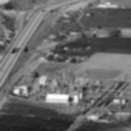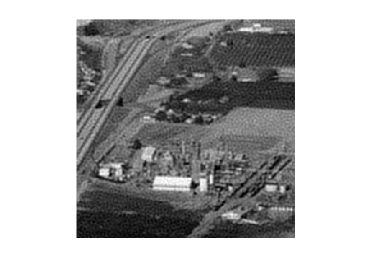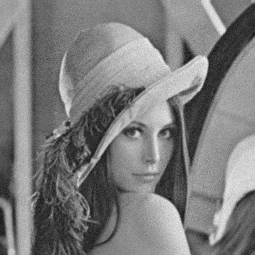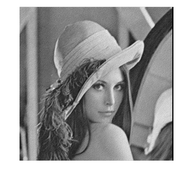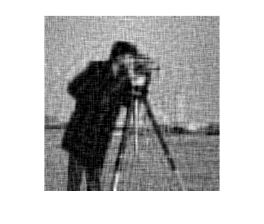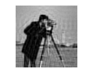Now we display the input image along with its deblurred and denoised pair.

Results

Denoise Lena direct method with \(\lambda = .06\)

Denoise Cameraman 25dB with direct method \(\lambda = .025\)

Denoise Cameraman 40dB with direct method \(\lambda = .025\)

Denoise Chemical Plant with \(\lambda = .1\)