Introduction
In the investigation of chaotic systems it is clear that hopes of predicting long term behavior is futile. However, from the investigation of chaotic systems Ergodic Theory has arisen in order to predict the average long term behavior of dynamic systems. It is our intent to investigate the theoretical results of a main result of Ergodic Theory, namely that of Birkhoff’s Ergodic Theorem.
Definition
An Ergodic Endomorphism or measure preserving map is a map \(T: X\rightarrow X\) where for measure \(\mu\) it is the case that \(T\) satisfies
- \(T\) is surjective
- \(T\) is measureable
- \(\mu(T^{-1}A)=\mu(A)\) for all \(A\) in the sigma algebra on \(X\), for preimage \(T^{-1}(A)\).
Birhoff’s Ergodic Theorem
Let \(T\) be an ergodic endomorphism of the probability space \(X\) with measure \(\mu\) and let \(f:X\rightarrow \mathbb{R}\) be a real-valued measurable function. Then for almost every \(x \in X\), we have
\(\lim_{n\rightarrow \infty} \frac{1}{n}\sum_{j=0}^{n}{f\circ T^j(x)} = \int_{X} f d\mu\)
A simple measureable function is the characteristic function \(f\) of some subset \(A\subset X\).
\[f(x)=\begin{cases} 1 & \text{ if }x\in A \\ 0 & \text{ if }x\not\in A \end{cases}\]
The statement of Birkhoff’s Theorem is that for almost all initial points, the time-wise average converges to the space-wise average. More precisely that is for all but a set of measure zero initial points \(x_0\), the average value over the ‘time evolution’ orbit of the point \(x_0\), given by \(\{T^j(x_0)\}\), is given by the invariant distribution \(\mu\).
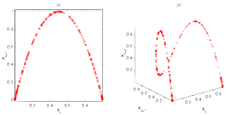
Logistic Maps
The family of logistic maps are maps, for some value \(r\in [0,4]\) are given by
\[T:[0,1] \rightarrow [0,1]\]
\[T(x) = r\cdot x (1-x)\]
These functions simulate the effects of reproduction for small populations and starvation at a population’s carrying capacity.
The logistic map for \(r=4\) is a well know ergodic endomorphism.
We define time evolutions of an initial point \(x_0\) at time \(t\) by
\(X_{t+1} = T(X_t)\)
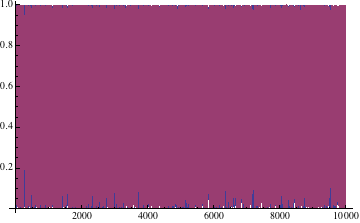
A graph of the evolution of the logistic map for \(r=4\) can be seen below.
 We may observer the chaotic behavior of the logistic map by selecting a random initial point \(X_0\) in the domain, and a second random point initial point \(X_0^{'}\) within some \(\epsilon=10^{-8}\) of \(X_0\).
We see that within 100 time iterations, the values of the two points have dispersed.
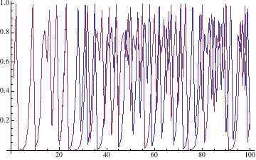
The residues of the points shows the dispersion of the points.
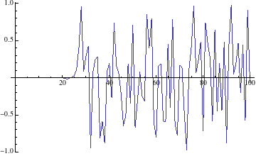
In the long term iterations of the map orbit the co-domain fast enough to fill the plot.
Calculating Invariant Distribution
The value of first investigating the logistic map is that it has an invariant distribution with may be calculated analytically, which leads into general methods for finding such a distribution.
Consider \(\mathbb{P}(X_{t+1}\le x)\), the cumulative distribution of the logistic map.
\(\begin{align*}
\mathbb{P}(X_{t+1}\le x) &= \mathbb{P}(X_{t+1}\in[0,x])= \mathbb{P}(X_{t}\in F^{-1}([0,x]))\\
&=\mathbb{P}(X_{t}\in [0,\frac{1}{2}(1-\sqrt{1-x})]\cup\frac{1}{2}([1+\sqrt{1-x},1])))\\
&=\int_0^{\frac{1}{2}(1-\sqrt{1-x})}\rho_t(y) dy+\int_{\frac{1}{2}(1+\sqrt{1-x})}^1\rho_t(y) dy
\end{align*}\)
Where \(\rho_t\) is the distribution of \(X_t\), this yields that
\(\int_0^x \rho_{t+1}(y)dy =\int_0^{\frac{1}{2}(1-\sqrt{1-x})} \rho_t(y) dy+ \int_{\frac{1}{2}(1+\sqrt{1-x})}^1 \rho_t (y) dy\)
In general this sort expression may be difficult or impossible to solve. The logistic map however, yields to the following method by differentiating both sides of the previous expression.
\(\begin{align*}
\rho_{t+1} &= \frac{d}{dx} \int_0^{\frac{1}{2}(1-\sqrt{1-x})} \rho_t(y) dy+ \frac{d}{dx}\int_{\frac{1}{2}(1+\sqrt{1-x})}^1 \rho_t (y) dy \\
&= \rho_t (\frac{1}{2}(1-\sqrt{1-x})) \frac{d}{dx}( \frac{1}{2}(1-\sqrt{1-x}))-\rho_t (\frac{1}{2}(1+\sqrt{1-x})) \frac{d}{dx}( \frac{1}{2}(1+\sqrt{1-x}))\\
&= \frac{1}{4\sqrt{1-x}} (\rho_t(\frac{1}{2}(1-\sqrt{1-x}))+ \rho_t(\frac{1}{2}(1+\sqrt{1-x})))
\end{align*}\)
First note that the previous display is an expression between distributions under iterations of the map. This expression is solvable and we may verify that \(\rho(x)=\frac{1}{\pi\sqrt{x(1-x)}}\) is the unique solution. We see that
\(\begin{align*}
\rho(\frac{1}{2}(1-\sqrt{1-x})) &= \frac{1}{pi}( \frac{1}{2}(1+\sqrt{1-x})(1-\frac{1}{2}(1+\sqrt{1-x})))^{-1/2}\\
&= \frac{1}{\pi}( \frac{1}{2}(1-\sqrt{1-x})\frac{1}{2}(1+\sqrt{1-x}))^{-1/2} = \frac{2}{\pi\sqrt{x}}
\end{align*}\)
Then by noting that \(\rho(x)=\rho(1-x)\) it follows that
\[\rho_{t+1} = \frac{1}{4\sqrt{1-x}} (\rho_t(\frac{1}{2}(1-\sqrt{1-x}))+ \rho_t(\frac{1}{2}(1+\sqrt{1-x})))
= \frac{1}{\pi\sqrt{x(1-x)}}=\rho_t\]
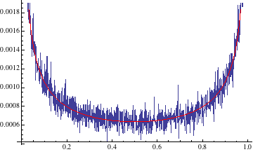
Comparing Time and Invariant Distribution
We may then plot the histogram produced by selecting a random initial position and evaluating the function over a period of several steps. Below we sample a random point in \([0,1]\) for 1 million steps then by breaking the domain into one thousand intervals we may approximate a histogram giving the distribution of the logistic function with respect to time. For comparison we plot our analytic invariant space solution.
The Perron-Frobenius Operator
The recurrent expression obtained in evaluating the invariant distribution of the Logistic map is a type of linear operator called a Perron-Frobenius Operator. These operators describe the time evolution of mappings in phase space defined such that for Perron-Frobenius operator \(P\), where the invariant distribtution satisfies
\[\rho_{t+1} = P\rho_{t} \quad \rho = P \rho\]
A description of the Perron-Frobenius operator is given explicitly as
\[P \rho(y) = \sum_{x\in T^{-1}(y)} \frac{\rho(x)}{|T^{'}(x)|}\]
We note that this is exactly the form of the expression we obtained in evaluating the invariant distribution of the Logistic map.
In their paper Klaus, Koltai, Sch{"u}tte \cite{PFO} give a numerical method adapted from Ulam’s Monte Carlo method. Ulam’s method is a projection from the Perron-Frobenius operator’s Banach space to a subspace spanned by indicator functions, of the type given as example in the introduction of the Birkhoff Ergodic Theorem. For simplicity we may simply split the codomain into \(N\) small intervals \(\mathbb{B}_i = [\frac{i}{N},\frac{i+1}{N}]\)
\[\mathbb{I}_{\mathbb{B}_i}(x)=\begin{cases} 1 & x\in \mathbb{B}_i \\ 0 & x\not\in \mathbb{B}_i \end{cases}\]
Then the Perron-Frobenius operator is given by
\[P=(p_{ij})\in \mathbb{R}^{k \times k}\]
\[p_{ij} = \frac{\mu(T^{-1}(\mathbb{B}_j)\cap \mathbb{B}_i)}{\mu(\mathbb{B}_i)}\]
For example
\[P_{\text{SOM}}=\small{\begin{pmatrix} 0 & 0.572 & 0.428 & 0 & 0 & 0 & 0 & 0 \\
0 & 0 & 1 & 0 & 0 & 0 & 0 & 0 \\
0 & 0 & 0 & 1 & 0 & 0 & 0 & 0 \\
0 & 0 & 0 & 0.394 & 0.606 & 0 & 0 & 0 \\
0 & 0 & 0 & 0 & 0.306 & 0.694 & 0 & 0 \\
0 & 0 & 0 & 0 & 0 & 0 & 0.697 & 0.303 \\
0 & 0 & 0 & 0 & 0 & 0.189 & 0.213 & 0.598 \\
0.202 & 0.204 & 0.195 & 0.2 & 0.199 & 0 & 0 & 0\end{pmatrix}}\]
The normalization of this discrete operator makes it the row-stochastic operator for a finite Markov chain.
This view of the operator allows us to approximate the matrix \((p_{ij})\) by sampling points in some interval \(\mathbb{B}_i\) and approximating the probability that a point will move into each interval \(\mathbb{B}_j\). So for \(L\) test points, and \(x_i^l\in \mathbb{B}_i\)
\(p_{ij}\approx \frac{1}{L} \sum^L_{l=1}\mathbb{I}_{\mathbb{B}_j}(T(x_i^l))\)
Then since \(\mu(T^{-1}(\mathbb{B}_j)\cap \mathbb{B}_i)= \int \mathbb{I}_{\mathbb{B}_j}\cdot P \mathbb{I}_{\mathbb{B}_i} d\mu\) is evaluated by the previous integral, this evaluation of each \(p_{ij}\) is a Monte-Carlo approximation.
Then finally for the matrix \(P=(p_{ij})\), we may evaluate the invariant distribution \(P\rho = \rho\) as the eigenvector giving the discrete distribution, for eigenvalue \(\lambda=1\).
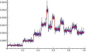
The Shobu-Ose-Mori Map
The Shobu-Ose-Mori map allows for a demonstration of the power of the discretization of the Perron-Frobenius operator. These maps are defined as
There is no analytic solution to the invariant distribution of these maps.
We see a fantastic display of the Birkhoff Ergodic Theorem as the time orbit of a point, whose histogram is shown below in blue, approximates the Perron-Frobenius numerical approximation of the invariant distribution, shown below in red.
Let \(\alpha =0.7\), \(\beta =0.2\), \(\gamma=0.8/(1+\alpha)\).
\[f(x)=\begin{cases} \alpha x +0.2 & 0\le x\le \gamma \\
\alpha^{-1}(x-0.8)+1 & \gamma\le x \le 0.8 \\
-\beta^{-1} (x-1) & 0.8 \le x\le 1 \end{cases}\]